\n",
"**Vectors and matrices in `numpy`** - Important implementation notes\n",
"\n",
"A vector in `numpy` is a one dimensional array, for example `np.array([1, 2, 3])` is a vector. A matrix in `numpy` is a two dimensional array, for example `np.array([[1, 2, 3], [4, 5, 6]])`. However, the following is still considered a matrix `np.array([[1, 2, 3]])` since it has two dimensions, even if it has a shape of 1x3 (which looks like a vector).\n",
"\n",
"Given the above, the function `np.dot` which we will use for all matrix/vector multiplication has the following properties:\n",
"- It always performs inner products on vectors. If `x=np.array([1, 2, 3])`, then `np.dot(x, x)` is a scalar.\n",
"- For matrix-vector multiplication, so if $X$ is a $m\\times n$ matrix and $y$ is a vector of length $m$, then the operation `np.dot(y, X)` considers $y$ as a $1 \\times m$ vector. On the other hand, if $y$ is a vector of length $n$, then the operation `np.dot(X, y)` considers $y$ as a $n \\times 1$ vector.\n",
"- A vector can be promoted to a matrix using `y[None]` or `[y[np.newaxis]`. That is, if `y = np.array([1, 2, 3])` is a vector of size 3, then `y[None, :]` is a matrix of shape $1 \\times 3$. We can use `y[:, None]` to obtain a shape of $3 \\times 1$.\n",
"
\n",
"
"
]
},
{
"cell_type": "code",
"execution_count": null,
"metadata": {},
"outputs": [],
"source": [
"def gradientDescent(X, y, theta, alpha, num_iters):\n",
" \"\"\"\n",
" Performs gradient descent to learn `theta`. Updates theta by taking `num_iters`\n",
" gradient steps with learning rate `alpha`.\n",
" \n",
" Parameters\n",
" ----------\n",
" X : array_like\n",
" The input dataset of shape (m x n+1).\n",
" \n",
" y : arra_like\n",
" Value at given features. A vector of shape (m, ).\n",
" \n",
" theta : array_like\n",
" Initial values for the linear regression parameters. \n",
" A vector of shape (n+1, ).\n",
" \n",
" alpha : float\n",
" The learning rate.\n",
" \n",
" num_iters : int\n",
" The number of iterations for gradient descent. \n",
" \n",
" Returns\n",
" -------\n",
" theta : array_like\n",
" The learned linear regression parameters. A vector of shape (n+1, ).\n",
" \n",
" J_history : list\n",
" A python list for the values of the cost function after each iteration.\n",
" \n",
" Instructions\n",
" ------------\n",
" Peform a single gradient step on the parameter vector theta.\n",
"\n",
" While debugging, it can be useful to print out the values of \n",
" the cost function (computeCost) and gradient here.\n",
" \"\"\"\n",
" # Initialize some useful values\n",
" m = y.shape[0] # number of training examples\n",
" \n",
" # make a copy of theta, to avoid changing the original array, since numpy arrays\n",
" # are passed by reference to functions\n",
" theta = theta.copy()\n",
" \n",
" J_history = [] # Use a python list to save cost in every iteration\n",
" \n",
" for i in range(num_iters):\n",
" # ==================== YOUR CODE HERE =================================\n",
" \n",
"\n",
" # =====================================================================\n",
" \n",
" # save the cost J in every iteration\n",
" J_history.append(computeCost(X, y, theta))\n",
" \n",
" return theta, J_history"
]
},
{
"cell_type": "markdown",
"metadata": {},
"source": [
"After you are finished call the implemented `gradientDescent` function and print the computed $\\theta$. We initialize the $\\theta$ parameters to 0 and the learning rate $\\alpha$ to 0.01. Execute the following cell to check your code."
]
},
{
"cell_type": "code",
"execution_count": null,
"metadata": {},
"outputs": [],
"source": [
"# initialize fitting parameters\n",
"theta = np.zeros(2)\n",
"\n",
"# some gradient descent settings\n",
"iterations = 1500\n",
"alpha = 0.01\n",
"\n",
"theta, J_history = gradientDescent(X ,y, theta, alpha, iterations)\n",
"print('Theta found by gradient descent: {:.4f}, {:.4f}'.format(*theta))\n",
"print('Expected theta values (approximately): [-3.6303, 1.1664]')"
]
},
{
"cell_type": "markdown",
"metadata": {},
"source": [
"We will use your final parameters to plot the linear fit. The results should look like the following figure.\n",
"\n",
""
]
},
{
"cell_type": "code",
"execution_count": null,
"metadata": {},
"outputs": [],
"source": [
"# plot the linear fit\n",
"plotData(X[:, 1], y)\n",
"pyplot.plot(X[:, 1], np.dot(X, theta), '-')\n",
"pyplot.legend(['Training data', 'Linear regression']);"
]
},
{
"cell_type": "markdown",
"metadata": {},
"source": [
"Your final values for $\\theta$ will also be used to make predictions on profits in areas of 35,000 and 70,000 people.\n",
"\n",
"
\n",
"Note the way that the following lines use matrix multiplication, rather than explicit summation or looping, to calculate the predictions. This is an example of code vectorization in `numpy`.\n",
"
\n",
"\n",
"
\n",
"Note that the first argument to the `numpy` function `dot` is a python list. `numpy` can internally converts **valid** python lists to numpy arrays when explicitly provided as arguments to `numpy` functions.\n",
"
\n"
]
},
{
"cell_type": "code",
"execution_count": null,
"metadata": {},
"outputs": [],
"source": [
"# Predict values for population sizes of 35,000 and 70,000\n",
"predict1 = np.dot([1, 3.5], theta)\n",
"print('For population = 35,000, we predict a profit of {:.2f}\\n'.format(predict1*10000))\n",
"\n",
"predict2 = np.dot([1, 7], theta)\n",
"print('For population = 70,000, we predict a profit of {:.2f}\\n'.format(predict2*10000))"
]
},
{
"cell_type": "markdown",
"metadata": {},
"source": [
"*You should now submit your solutions by executing the next cell.*"
]
},
{
"cell_type": "code",
"execution_count": null,
"metadata": {},
"outputs": [],
"source": [
"grader[3] = gradientDescent\n",
"grader.grade()"
]
},
{
"cell_type": "markdown",
"metadata": {},
"source": [
"### 2.4 Visualizing $J(\\theta)$\n",
"\n",
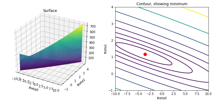
"To understand the cost function $J(\\theta)$ better, you will now plot the cost over a 2-dimensional grid of $\\theta_0$ and $\\theta_1$ values. You will not need to code anything new for this part, but you should understand how the code you have written already is creating these images.\n",
"\n",
"In the next cell, the code is set up to calculate $J(\\theta)$ over a grid of values using the `computeCost` function that you wrote. After executing the following cell, you will have a 2-D array of $J(\\theta)$ values. Then, those values are used to produce surface and contour plots of $J(\\theta)$ using the matplotlib `plot_surface` and `contourf` functions. The plots should look something like the following:\n",
"\n",
"\n",
"\n",
"The purpose of these graphs is to show you how $J(\\theta)$ varies with changes in $\\theta_0$ and $\\theta_1$. The cost function $J(\\theta)$ is bowl-shaped and has a global minimum. (This is easier to see in the contour plot than in the 3D surface plot). This minimum is the optimal point for $\\theta_0$ and $\\theta_1$, and each step of gradient descent moves closer to this point."
]
},
{
"cell_type": "code",
"execution_count": null,
"metadata": {},
"outputs": [],
"source": [
"# grid over which we will calculate J\n",
"theta0_vals = np.linspace(-10, 10, 100)\n",
"theta1_vals = np.linspace(-1, 4, 100)\n",
"\n",
"# initialize J_vals to a matrix of 0's\n",
"J_vals = np.zeros((theta0_vals.shape[0], theta1_vals.shape[0]))\n",
"\n",
"# Fill out J_vals\n",
"for i, theta0 in enumerate(theta0_vals):\n",
" for j, theta1 in enumerate(theta1_vals):\n",
" J_vals[i, j] = computeCost(X, y, [theta0, theta1])\n",
" \n",
"# Because of the way meshgrids work in the surf command, we need to\n",
"# transpose J_vals before calling surf, or else the axes will be flipped\n",
"J_vals = J_vals.T\n",
"\n",
"# surface plot\n",
"fig = pyplot.figure(figsize=(12, 5))\n",
"ax = fig.add_subplot(121, projection='3d')\n",
"ax.plot_surface(theta0_vals, theta1_vals, J_vals, cmap='viridis')\n",
"pyplot.xlabel('theta0')\n",
"pyplot.ylabel('theta1')\n",
"pyplot.title('Surface')\n",
"\n",
"# contour plot\n",
"# Plot J_vals as 15 contours spaced logarithmically between 0.01 and 100\n",
"ax = pyplot.subplot(122)\n",
"pyplot.contour(theta0_vals, theta1_vals, J_vals, linewidths=2, cmap='viridis', levels=np.logspace(-2, 3, 20))\n",
"pyplot.xlabel('theta0')\n",
"pyplot.ylabel('theta1')\n",
"pyplot.plot(theta[0], theta[1], 'ro', ms=10, lw=2)\n",
"pyplot.title('Contour, showing minimum')\n",
"pass"
]
},
{
"cell_type": "markdown",
"metadata": {},
"source": [
"## Optional Exercises\n",
"\n",
"If you have successfully completed the material above, congratulations! You now understand linear regression and should able to start using it on your own datasets.\n",
"\n",
"For the rest of this programming exercise, we have included the following optional exercises. These exercises will help you gain a deeper understanding of the material, and if you are able to do so, we encourage you to complete them as well. You can still submit your solutions to these exercises to check if your answers are correct.\n",
"\n",
"## 3 Linear regression with multiple variables\n",
"\n",
"In this part, you will implement linear regression with multiple variables to predict the prices of houses. Suppose you are selling your house and you want to know what a good market price would be. One way to do this is to first collect information on recent houses sold and make a model of housing prices.\n",
"\n",
"The file `Data/ex1data2.txt` contains a training set of housing prices in Portland, Oregon. The first column is the size of the house (in square feet), the second column is the number of bedrooms, and the third column is the price\n",
"of the house. \n",
"\n",
"
\n",
"### 3.1 Feature Normalization\n",
"\n",
"We start by loading and displaying some values from this dataset. By looking at the values, note that house sizes are about 1000 times the number of bedrooms. When features differ by orders of magnitude, first performing feature scaling can make gradient descent converge much more quickly."
]
},
{
"cell_type": "code",
"execution_count": null,
"metadata": {},
"outputs": [],
"source": [
"# Load data\n",
"data = np.loadtxt(os.path.join('Data', 'ex1data2.txt'), delimiter=',')\n",
"X = data[:, :2]\n",
"y = data[:, 2]\n",
"m = y.size\n",
"\n",
"# print out some data points\n",
"print('{:>8s}{:>8s}{:>10s}'.format('X[:,0]', 'X[:, 1]', 'y'))\n",
"print('-'*26)\n",
"for i in range(10):\n",
" print('{:8.0f}{:8.0f}{:10.0f}'.format(X[i, 0], X[i, 1], y[i]))"
]
},
{
"cell_type": "markdown",
"metadata": {},
"source": [
"Your task here is to complete the code in `featureNormalize` function:\n",
"- Subtract the mean value of each feature from the dataset.\n",
"- After subtracting the mean, additionally scale (divide) the feature values by their respective “standard deviations.”\n",
"\n",
"The standard deviation is a way of measuring how much variation there is in the range of values of a particular feature (most data points will lie within ±2 standard deviations of the mean); this is an alternative to taking the range of values (max-min). In `numpy`, you can use the `std` function to compute the standard deviation. \n",
"\n",
"For example, the quantity `X[:, 0]` contains all the values of $x_1$ (house sizes) in the training set, so `np.std(X[:, 0])` computes the standard deviation of the house sizes.\n",
"At the time that the function `featureNormalize` is called, the extra column of 1’s corresponding to $x_0 = 1$ has not yet been added to $X$. \n",
"\n",
"You will do this for all the features and your code should work with datasets of all sizes (any number of features / examples). Note that each column of the matrix $X$ corresponds to one feature.\n",
"\n",
"
\n",
"**Implementation Note:** When normalizing the features, it is important\n",
"to store the values used for normalization - the mean value and the standard deviation used for the computations. After learning the parameters\n",
"from the model, we often want to predict the prices of houses we have not\n",
"seen before. Given a new x value (living room area and number of bedrooms), we must first normalize x using the mean and standard deviation that we had previously computed from the training set.\n",
"
\n",
"
"
]
},
{
"cell_type": "code",
"execution_count": null,
"metadata": {},
"outputs": [],
"source": [
"def featureNormalize(X):\n",
" \"\"\"\n",
" Normalizes the features in X. returns a normalized version of X where\n",
" the mean value of each feature is 0 and the standard deviation\n",
" is 1. This is often a good preprocessing step to do when working with\n",
" learning algorithms.\n",
" \n",
" Parameters\n",
" ----------\n",
" X : array_like\n",
" The dataset of shape (m x n).\n",
" \n",
" Returns\n",
" -------\n",
" X_norm : array_like\n",
" The normalized dataset of shape (m x n).\n",
" \n",
" Instructions\n",
" ------------\n",
" First, for each feature dimension, compute the mean of the feature\n",
" and subtract it from the dataset, storing the mean value in mu. \n",
" Next, compute the standard deviation of each feature and divide\n",
" each feature by it's standard deviation, storing the standard deviation \n",
" in sigma. \n",
" \n",
" Note that X is a matrix where each column is a feature and each row is\n",
" an example. You needto perform the normalization separately for each feature. \n",
" \n",
" Hint\n",
" ----\n",
" You might find the 'np.mean' and 'np.std' functions useful.\n",
" \"\"\"\n",
" # You need to set these values correctly\n",
" X_norm = X.copy()\n",
" mu = np.zeros(X.shape[1])\n",
" sigma = np.zeros(X.shape[1])\n",
"\n",
" # =========================== YOUR CODE HERE =====================\n",
"\n",
" \n",
" # ================================================================\n",
" return X_norm, mu, sigma"
]
},
{
"cell_type": "markdown",
"metadata": {},
"source": [
"Execute the next cell to run the implemented `featureNormalize` function."
]
},
{
"cell_type": "code",
"execution_count": null,
"metadata": {},
"outputs": [],
"source": [
"# call featureNormalize on the loaded data\n",
"X_norm, mu, sigma = featureNormalize(X)\n",
"\n",
"print('Computed mean:', mu)\n",
"print('Computed standard deviation:', sigma)"
]
},
{
"cell_type": "markdown",
"metadata": {},
"source": [
"*You should not submit your solutions.*"
]
},
{
"cell_type": "code",
"execution_count": null,
"metadata": {},
"outputs": [],
"source": [
"grader[4] = featureNormalize\n",
"grader.grade()"
]
},
{
"cell_type": "markdown",
"metadata": {},
"source": [
"After the `featureNormalize` function is tested, we now add the intercept term to `X_norm`:"
]
},
{
"cell_type": "code",
"execution_count": null,
"metadata": {},
"outputs": [],
"source": [
"# Add intercept term to X\n",
"X = np.concatenate([np.ones((m, 1)), X_norm], axis=1)"
]
},
{
"cell_type": "markdown",
"metadata": {},
"source": [
"
\n",
"### 3.2 Gradient Descent\n",
"\n",
"Previously, you implemented gradient descent on a univariate regression problem. The only difference now is that there is one more feature in the matrix $X$. The hypothesis function and the batch gradient descent update\n",
"rule remain unchanged. \n",
"\n",
"You should complete the code for the functions `computeCostMulti` and `gradientDescentMulti` to implement the cost function and gradient descent for linear regression with multiple variables. If your code in the previous part (single variable) already supports multiple variables, you can use it here too.\n",
"Make sure your code supports any number of features and is well-vectorized.\n",
"You can use the `shape` property of `numpy` arrays to find out how many features are present in the dataset.\n",
"\n",
"
\n",
"**Implementation Note:** In the multivariate case, the cost function can\n",
"also be written in the following vectorized form:\n",
"\n",
"$$ J(\\theta) = \\frac{1}{2m}(X\\theta - \\vec{y})^T(X\\theta - \\vec{y}) $$\n",
"\n",
"where \n",
"\n",
"$$ X = \\begin{pmatrix}\n",
" - (x^{(1)})^T - \\\\\n",
" - (x^{(2)})^T - \\\\\n",
" \\vdots \\\\\n",
" - (x^{(m)})^T - \\\\ \\\\\n",
" \\end{pmatrix} \\qquad \\mathbf{y} = \\begin{bmatrix} y^{(1)} \\\\ y^{(2)} \\\\ \\vdots \\\\ y^{(m)} \\\\\\end{bmatrix}$$\n",
"\n",
"the vectorized version is efficient when you are working with numerical computing tools like `numpy`. If you are an expert with matrix operations, you can prove to yourself that the two forms are equivalent.\n",
"
\n",
"\n",
"
"
]
},
{
"cell_type": "code",
"execution_count": null,
"metadata": {},
"outputs": [],
"source": [
"def computeCostMulti(X, y, theta):\n",
" \"\"\"\n",
" Compute cost for linear regression with multiple variables.\n",
" Computes the cost of using theta as the parameter for linear regression to fit the data points in X and y.\n",
" \n",
" Parameters\n",
" ----------\n",
" X : array_like\n",
" The dataset of shape (m x n+1).\n",
" \n",
" y : array_like\n",
" A vector of shape (m, ) for the values at a given data point.\n",
" \n",
" theta : array_like\n",
" The linear regression parameters. A vector of shape (n+1, )\n",
" \n",
" Returns\n",
" -------\n",
" J : float\n",
" The value of the cost function. \n",
" \n",
" Instructions\n",
" ------------\n",
" Compute the cost of a particular choice of theta. You should set J to the cost.\n",
" \"\"\"\n",
" # Initialize some useful values\n",
" m = y.shape[0] # number of training examples\n",
" \n",
" # You need to return the following variable correctly\n",
" J = 0\n",
" \n",
" # ======================= YOUR CODE HERE ===========================\n",
"\n",
" \n",
" # ==================================================================\n",
" return J\n"
]
},
{
"cell_type": "markdown",
"metadata": {},
"source": [
"*You should now submit your solutions.*"
]
},
{
"cell_type": "code",
"execution_count": null,
"metadata": {},
"outputs": [],
"source": [
"grader[5] = computeCostMulti\n",
"grader.grade()"
]
},
{
"cell_type": "markdown",
"metadata": {},
"source": [
"
"
]
},
{
"cell_type": "code",
"execution_count": null,
"metadata": {},
"outputs": [],
"source": [
"def gradientDescentMulti(X, y, theta, alpha, num_iters):\n",
" \"\"\"\n",
" Performs gradient descent to learn theta.\n",
" Updates theta by taking num_iters gradient steps with learning rate alpha.\n",
" \n",
" Parameters\n",
" ----------\n",
" X : array_like\n",
" The dataset of shape (m x n+1).\n",
" \n",
" y : array_like\n",
" A vector of shape (m, ) for the values at a given data point.\n",
" \n",
" theta : array_like\n",
" The linear regression parameters. A vector of shape (n+1, )\n",
" \n",
" alpha : float\n",
" The learning rate for gradient descent. \n",
" \n",
" num_iters : int\n",
" The number of iterations to run gradient descent. \n",
" \n",
" Returns\n",
" -------\n",
" theta : array_like\n",
" The learned linear regression parameters. A vector of shape (n+1, ).\n",
" \n",
" J_history : list\n",
" A python list for the values of the cost function after each iteration.\n",
" \n",
" Instructions\n",
" ------------\n",
" Peform a single gradient step on the parameter vector theta.\n",
"\n",
" While debugging, it can be useful to print out the values of \n",
" the cost function (computeCost) and gradient here.\n",
" \"\"\"\n",
" # Initialize some useful values\n",
" m = y.shape[0] # number of training examples\n",
" \n",
" # make a copy of theta, which will be updated by gradient descent\n",
" theta = theta.copy()\n",
" \n",
" J_history = []\n",
" \n",
" for i in range(num_iters):\n",
" # ======================= YOUR CODE HERE ==========================\n",
"\n",
" \n",
" # =================================================================\n",
" \n",
" # save the cost J in every iteration\n",
" J_history.append(computeCostMulti(X, y, theta))\n",
" \n",
" return theta, J_history"
]
},
{
"cell_type": "markdown",
"metadata": {},
"source": [
"*You should now submit your solutions.*"
]
},
{
"cell_type": "code",
"execution_count": null,
"metadata": {},
"outputs": [],
"source": [
"grader[6] = gradientDescentMulti\n",
"grader.grade()"
]
},
{
"cell_type": "markdown",
"metadata": {},
"source": [
"#### 3.2.1 Optional (ungraded) exercise: Selecting learning rates\n",
"\n",
"In this part of the exercise, you will get to try out different learning rates for the dataset and find a learning rate that converges quickly. You can change the learning rate by modifying the following code and changing the part of the code that sets the learning rate.\n",
"\n",
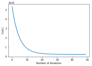
"Use your implementation of `gradientDescentMulti` function and run gradient descent for about 50 iterations at the chosen learning rate. The function should also return the history of $J(\\theta)$ values in a vector $J$.\n",
"\n",
"After the last iteration, plot the J values against the number of the iterations.\n",
"\n",
"If you picked a learning rate within a good range, your plot look similar as the following Figure. \n",
"\n",
"\n",
"\n",
"If your graph looks very different, especially if your value of $J(\\theta)$ increases or even blows up, adjust your learning rate and try again. We recommend trying values of the learning rate $\\alpha$ on a log-scale, at multiplicative steps of about 3 times the previous value (i.e., 0.3, 0.1, 0.03, 0.01 and so on). You may also want to adjust the number of iterations you are running if that will help you see the overall trend in the curve.\n",
"\n",
"
\n",
"**Implementation Note:** If your learning rate is too large, $J(\\theta)$ can diverge and ‘blow up’, resulting in values which are too large for computer calculations. In these situations, `numpy` will tend to return\n",
"NaNs. NaN stands for ‘not a number’ and is often caused by undefined operations that involve −∞ and +∞.\n",
"
\n",
"\n",
"
\n",
"**MATPLOTLIB tip:** To compare how different learning learning rates affect convergence, it is helpful to plot $J$ for several learning rates on the same figure. This can be done by making `alpha` a python list, and looping across the values within this list, and calling the plot function in every iteration of the loop. It is also useful to have a legend to distinguish the different lines within the plot. Search online for `pyplot.legend` for help on showing legends in `matplotlib`.\n",
"
\n",
"\n",
"Notice the changes in the convergence curves as the learning rate changes. With a small learning rate, you should find that gradient descent takes a very long time to converge to the optimal value. Conversely, with a large learning rate, gradient descent might not converge or might even diverge!\n",
"Using the best learning rate that you found, run the script\n",
"to run gradient descent until convergence to find the final values of $\\theta$. Next,\n",
"use this value of $\\theta$ to predict the price of a house with 1650 square feet and\n",
"3 bedrooms. You will use value later to check your implementation of the normal equations. Don’t forget to normalize your features when you make this prediction!"
]
},
{
"cell_type": "code",
"execution_count": null,
"metadata": {},
"outputs": [],
"source": [
"\"\"\"\n",
"Instructions\n",
"------------\n",
"We have provided you with the following starter code that runs\n",
"gradient descent with a particular learning rate (alpha). \n",
"\n",
"Your task is to first make sure that your functions - `computeCost`\n",
"and `gradientDescent` already work with this starter code and\n",
"support multiple variables.\n",
"\n",
"After that, try running gradient descent with different values of\n",
"alpha and see which one gives you the best result.\n",
"\n",
"Finally, you should complete the code at the end to predict the price\n",
"of a 1650 sq-ft, 3 br house.\n",
"\n",
"Hint\n",
"----\n",
"At prediction, make sure you do the same feature normalization.\n",
"\"\"\"\n",
"# Choose some alpha value - change this\n",
"alpha = 0.1\n",
"num_iters = 400\n",
"\n",
"# init theta and run gradient descent\n",
"theta = np.zeros(3)\n",
"theta, J_history = gradientDescentMulti(X, y, theta, alpha, num_iters)\n",
"\n",
"# Plot the convergence graph\n",
"pyplot.plot(np.arange(len(J_history)), J_history, lw=2)\n",
"pyplot.xlabel('Number of iterations')\n",
"pyplot.ylabel('Cost J')\n",
"\n",
"# Display the gradient descent's result\n",
"print('theta computed from gradient descent: {:s}'.format(str(theta)))\n",
"\n",
"# Estimate the price of a 1650 sq-ft, 3 br house\n",
"# ======================= YOUR CODE HERE ===========================\n",
"# Recall that the first column of X is all-ones. \n",
"# Thus, it does not need to be normalized.\n",
"\n",
"price = 0 # You should change this\n",
"\n",
"# ===================================================================\n",
"\n",
"print('Predicted price of a 1650 sq-ft, 3 br house (using gradient descent): ${:.0f}'.format(price))"
]
},
{
"cell_type": "markdown",
"metadata": {},
"source": [
"*You do not need to submit any solutions for this optional (ungraded) part.*"
]
},
{
"cell_type": "markdown",
"metadata": {},
"source": [
"
\n",
"### 3.3 Normal Equations\n",
"\n",
"In the lecture videos, you learned that the closed-form solution to linear regression is\n",
"\n",
"$$ \\theta = \\left( X^T X\\right)^{-1} X^T\\vec{y}$$\n",
"\n",
"Using this formula does not require any feature scaling, and you will get an exact solution in one calculation: there is no “loop until convergence” like in gradient descent. \n",
"\n",
"First, we will reload the data to ensure that the variables have not been modified. Remember that while you do not need to scale your features, we still need to add a column of 1’s to the $X$ matrix to have an intercept term ($\\theta_0$). The code in the next cell will add the column of 1’s to X for you."
]
},
{
"cell_type": "code",
"execution_count": null,
"metadata": {},
"outputs": [],
"source": [
"# Load data\n",
"data = np.loadtxt(os.path.join('Data', 'ex1data2.txt'), delimiter=',')\n",
"X = data[:, :2]\n",
"y = data[:, 2]\n",
"m = y.size\n",
"X = np.concatenate([np.ones((m, 1)), X], axis=1)"
]
},
{
"cell_type": "markdown",
"metadata": {},
"source": [
"Complete the code for the function `normalEqn` below to use the formula above to calculate $\\theta$. \n",
"\n",
"
"
]
},
{
"cell_type": "code",
"execution_count": null,
"metadata": {},
"outputs": [],
"source": [
"def normalEqn(X, y):\n",
" \"\"\"\n",
" Computes the closed-form solution to linear regression using the normal equations.\n",
" \n",
" Parameters\n",
" ----------\n",
" X : array_like\n",
" The dataset of shape (m x n+1).\n",
" \n",
" y : array_like\n",
" The value at each data point. A vector of shape (m, ).\n",
" \n",
" Returns\n",
" -------\n",
" theta : array_like\n",
" Estimated linear regression parameters. A vector of shape (n+1, ).\n",
" \n",
" Instructions\n",
" ------------\n",
" Complete the code to compute the closed form solution to linear\n",
" regression and put the result in theta.\n",
" \n",
" Hint\n",
" ----\n",
" Look up the function `np.linalg.pinv` for computing matrix inverse.\n",
" \"\"\"\n",
" theta = np.zeros(X.shape[1])\n",
" \n",
" # ===================== YOUR CODE HERE ============================\n",
"\n",
" \n",
" # =================================================================\n",
" return theta"
]
},
{
"cell_type": "markdown",
"metadata": {},
"source": [
"*You should now submit your solutions.*"
]
},
{
"cell_type": "code",
"execution_count": null,
"metadata": {},
"outputs": [],
"source": [
"grader[7] = normalEqn\n",
"grader.grade()"
]
},
{
"cell_type": "markdown",
"metadata": {},
"source": [
"Optional (ungraded) exercise: Now, once you have found $\\theta$ using this\n",
"method, use it to make a price prediction for a 1650-square-foot house with\n",
"3 bedrooms. You should find that gives the same predicted price as the value\n",
"you obtained using the model fit with gradient descent (in Section 3.2.1)."
]
},
{
"cell_type": "code",
"execution_count": null,
"metadata": {},
"outputs": [],
"source": [
"# Calculate the parameters from the normal equation\n",
"theta = normalEqn(X, y);\n",
"\n",
"# Display normal equation's result\n",
"print('Theta computed from the normal equations: {:s}'.format(str(theta)));\n",
"\n",
"# Estimate the price of a 1650 sq-ft, 3 br house\n",
"# ====================== YOUR CODE HERE ======================\n",
"\n",
"price = 0 # You should change this\n",
"\n",
"# ============================================================\n",
"\n",
"print('Predicted price of a 1650 sq-ft, 3 br house (using normal equations): ${:.0f}'.format(price))"
]
}
],
"metadata": {
"kernelspec": {
"display_name": "Python 3",
"language": "python",
"name": "python3"
},
"language_info": {
"codemirror_mode": {
"name": "ipython",
"version": 3
},
"file_extension": ".py",
"mimetype": "text/x-python",
"name": "python",
"nbconvert_exporter": "python",
"pygments_lexer": "ipython3",
"version": "3.6.4"
}
},
"nbformat": 4,
"nbformat_minor": 2
}